One of the reasons you may wish to do a hypothesis test is to determine whether there is a statistically significant difference between means, either for a single sample (in which case you would compare to a constant value) or for multiple independent or related samples (in which case you would compare between these different samples). Depending on the exact nature of the analysis different tests are required, and this page details the process for performing some of the most common ones using SPSS.
A question you may wish to ask of the wider population is: Does this sample come from a population where the mean summer daily energy consumption is \(19\)kWh?
This question can be answered by following the recommended steps, as follows:
While the first three assumptions should be met during the design and data collection phases, the fourth assumption should be checked at this stage (for instructions on doing this in SPSS, see the The normal distribution page of this module). If the normality assumption is not met you can try transforming the data or conducting the One sample Wilcoxon signed-rank test instead (you can also use this test if you have an ordinal rather than continuous variable).
The output should look like this:


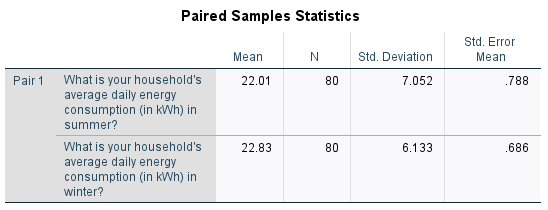
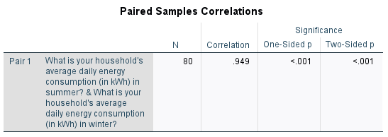
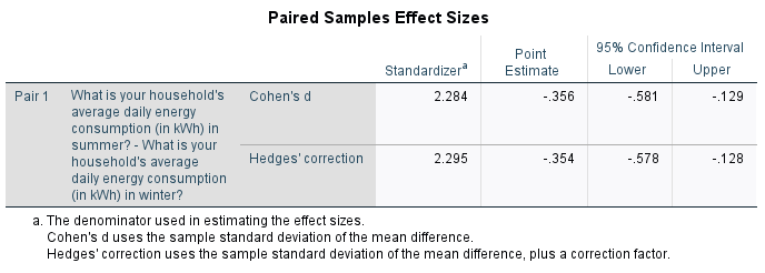
A question you may wish to ask of the wider population is: Is there a statistically significant difference between mean summer daily energy consumption and mean winter daily energy consumption?
This question can be answered by following the recommended steps, as follows:
While the first three assumptions should be met during the design and data collection phases, the fourth assumption should be checked at this stage (for instructions on doing this in SPSS, see the The normal distribution and Transformations pages of this module). If the normality assumption is not met you can try transforming the data or conducting the Wilcoxon signed rank test instead. You can also use this test if you have ordinal rather than continuous variables.
The output should look like this:

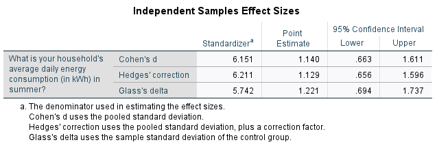
A question you may wish to ask of the wider population is: Is there a statistically significant difference in mean summer daily energy consumption for those with and without children?
This question can be answered by following the recommended steps, as follows:
While the first three assumptions should be met during the design and data collection phases, the fourth assumption should be checked at this stage (for instructions on doing this in SPSS, see the The normal distribution page of this module). If the normality assumption is not met you can try transforming the data or conducting the Mann-Whitney U test instead. You can also use this test if you have an ordinal rather than continuous dependent variable.
The output should look like this:


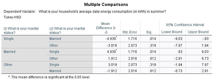
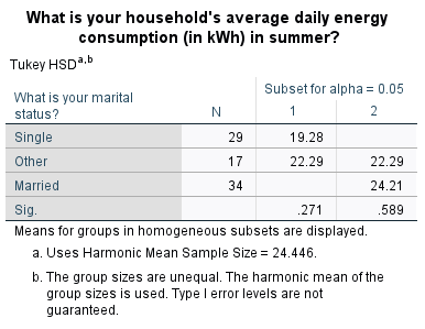
A question you may wish to ask of the wider population is: Is there a statistically significant difference in mean summer daily energy consumption for any of the different marital statuses?
This question can be answered by following the recommended steps, as follows:
While the first three assumptions should be met during the design and data collection phases, the fourth and fifth assumptions should be checked at this stage (for instructions on checking the normality assumption in SPSS, see the The normal distribution page of this module). Instructions on checking the equal variances assumption are included in the analysis stage.
If the normality assumption is not met you can try transforming the data or conducting the Kruskall-Wallis one-way ANOVA instead. You can also use this test if you have an ordinal rather than continuous dependent variable. If the equal variances assumption is violated you will need to use a Welch or Brown-Forsythe statistic instead.
The output should look like this:


